[BDA 데이터 분석 모델링반 (ML 1) 15회차] 의사결정 트리(DT) 실습
DT 모델의 하이퍼파라미터를 알아보고, iris 데이터를 활용하여 DT 모델을 실습해본다.
DT 모델 하이퍼파라미터
criterion
분할 품질을 측정하는 기능
분류 (DecisionTreeClassifier): "gini" (기본값), "entropy"
회귀 (DecisionTreeRegressor): "squared_error" (기본값), "friedman_mse", "absolute_error", "poisson"
splitter
각 노드에서 분할을 선택하는 전략
"best" (기본값): 최적의 분할을 선택
"random": 무작위 분할을 선택
max_depth
트리의 최대 깊이로, 깊이가 깊으면 모델이 과적합될 수 있다.
기본값: None (노드가 순수해질 때까지 또는 min_samples_split보다 작은 샘플이 될 때까지 분할)
min_samples_split
내부 노드를 분할하는 데 필요한 최소 샘플 수
정수: 최소 샘플 수
부동소수점: 0.0과 1.0 사이의 비율 (전체 샘플 수에 대한)
min_samples_leaf
리프 노드에 있어야 하는 최소 샘플 수
정수: 최소 샘플 수
부동소수점: 0.0과 1.0 사이의 비율 (전체 샘플 수에 대한)
min_weight_fraction_leaf
리프 노드에 있어야 하는 최소 가중치 샘플의 비율로, 샘플 가중치가 있는 경우 사용된다.
기본값: 0.0
max_features
각 분할에서 고려할 최대 특징 수
정수: 최대 특징 수
부동소수점: 0.0과 1.0 사이의 비율 (전체 특징 수에 대한)
"auto", "sqrt", "log2", None
random_state
무작위성의 시드를 설정한다.
정수: 시드 값
None (기본값)
max_leaf_nodes
리프 노드의 최대 수로, 최적의 리프 노드 수를 찾는 데 사용된다.
기본값: None
min_impurity_decrease
분할이 유용하기 위해 필요한 최소 불순물 감소량
기본값: 0.0
class_weight
클래스 가중치로, 클래스 불균형을 처리하는 데 사용된다.
None (기본값), balanced, 딕셔너리
ccp_alpha
비용 복잡도 가지치기(최소 비용 복잡도 가지치기) 매개변수입니다.
기본값: 0.0
import numpy as np
import matplotlib.pyplot as plt

# 데이터셋 생성 (2차원)
np.random.seed(42)
X = np.vstack((np.random.normal([2, 2], 1, (50, 2)), np.random.normal([6, 6], 1, (50, 2))))
y = np.hstack((np.zeros(50), np.ones(50)))

# 데이터 시각화
plt.scatter(X[:, 0], X[:, 1], c=y, cmap='bwr', edgecolor='k')
plt.xlabel('Feature 1')
plt.ylabel('Feature 2')
plt.title('Synthetic Binary Classification Dataset')
plt.show()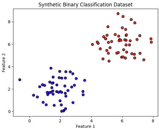
# 엔트로피 계산 함수
def entropy(y):
    classes, counts = np.unique(y, return_counts=True)
    probabilities = counts / len(y)
    return -np.sum([p * np.log2(p) for p in probabilities if p > 0])

# 지니 지수 계산 함수
def gini_index(y):
    classes, counts = np.unique(y, return_counts=True)
    probabilities = counts / len(y)
    return 1 - np.sum([p ** 2 for p in probabilities])
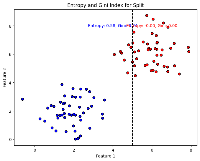
# 데이터셋 분할
threshold = 5
left_mask = X[:, 0] <= threshold
right_mask = X[:, 0] > threshold

X_left, y_left = X[left_mask], y[left_mask]
X_right, y_right = X[right_mask], y[right_mask]

# 엔트로피 및 지니 지수 계산
entropy_left = entropy(y_left)
entropy_right = entropy(y_right)
gini_left = gini_index(y_left)
gini_right = gini_index(y_right)

# 결과 출력
print(f'Left node - Entropy: {entropy_left:.4f}, Gini Index: {gini_left:.4f}')
print(f'Right node - Entropy: {entropy_right:.4f}, Gini Index: {gini_right:.4f}')

# 시각화
fig, ax = plt.subplots(1, 1, figsize=(8, 6))
ax.scatter(X[:, 0], X[:, 1], c=y, cmap='bwr', edgecolor='k')
ax.axvline(x=threshold, color='k', linestyle='--')
ax.text(threshold - 1, 8, f'Entropy: {entropy_left:.2f}, Gini: {gini_left:.2f}',
        verticalalignment='center', horizontalalignment='center', color='blue')
ax.text(threshold + 1, 8, f'Entropy: {entropy_right:.2f}, Gini: {gini_right:.2f}',
        verticalalignment='center', horizontalalignment='center', color='red')
ax.set_xlabel('Feature 1')
ax.set_ylabel('Feature 2')
ax.set_title('Entropy and Gini Index for Split')
plt.show()

'''
Left node - Entropy: 0.5788, Gini Index: 0.2378
Right node - Entropy: -0.0000, Gini Index: 0.0000
'''
# 예제 실행: Iris 데이터셋을 사용하여 트리 학습 및 평가
from sklearn.datasets import load_iris
from sklearn.model_selection import train_test_split

# 데이터셋 로드
iris = load_iris()
X, y = iris.data, iris.target
## DT를 학습시키기 위해서 필요한 함수
## 엔트로피, 지니계수
def entropy(y):
#y 클래스의 분포를 계산
classes, counts =np.unique(y, return_counts=True)
# 각 클래스들의 확률 계산
probabilities=counts/len(y)
#엔트로피 계산 : 각 클래스에 확률에 로그 값을 곱한 후 음수 부호 붙여서 합산
return -np.sum([p * np.log2(p) for p in probabilities if p > 0])
# 지니계수
def gini_index(y):
#y 클래스의 분포를 계산
classes, counts =np.unique(y, return_counts=True)
# 각 클래스들의 확률 계산
probabilities=counts/len(y)
# 지니 계수 : 각 클래스의 확률의 제곱 값을 합산한 후 1 에서 빼는 것
return 1 - np.sum([p ** 2 for p in probabilities])
##데이터의 분할 함수
def split_dataset(X,y,feature_index, threshold):
#데이터의 특성이랑 임계값에 따라 데이터를 좌우로 나눈다.
left_mask=X[:, feature_index] <=threshold
right_mask=X[:, feature_index] >threshold
return X[left_mask], y[left_mask], X[right_mask], y[right_mask]
##분할시 최적의 분할을 찾아야 한다.
##임계값에 분할하면서 분할된 노드의 불순도들 계산
## gini, entropy로 계산
## 더 낮은 점수인지 따라서 분할 갱신한다.
def best_split(X,y, criterion='gini'):
best_score= float('inf') # 초기 점수 설정
best_feature = None # 최적의 인덱스 초기화
best_threshold = None # 최적의 임계값 초기화
# 각 피처에 대한 분할 시도
# 반복문을 통해 X피처에 대한 분할 시도
for feature_index in range(X.shape[1]):
# 각 특성의 고유한 값들에 대한 분할 기준 시도
# 임계점을 정해야 하는 것
thresholds=np.unique(X[:, feature_index])
for threshold in thresholds:
X_left, y_left, X_right, y_right =split_dataset(X,y,feature_index,threshold)
#유효하지 않은 분할은 건너 뛰는 경우
if len(y_left)==0 or len(y_right)==0:
continue
#분할된 노드의 불순도 계산
if criterion =='gini':
score =(len(y_left)* gini_index(y_left) + len(y_right)*gini_index(y_right)) /len(y)
elif criterion =='entropy':
score =(len(y_left)* entropy(y_left) + len(y_right)*entropy(y_right)) /len(y)
# 분할에 대한 갱신이 필요하다.
if score < best_score:
best_score = score
best_feature = feature_index
best_threshold = threshold
#최적값을 갱신한다.
return best_feature, best_threshold
## 의사결정나무 트리 기준으로해서 분할을 최적으로 찾아야 한다. 쭉 내려가면서 더 이상 분할할 수 없는 리프 노드까지 내려가는 것
## 의사결정나무 노드 정의
class DecisionTreeNode:
def __init__(self, feature=None, threshold=None, left=None, right=None, value=None):
self.feature = feature # 분할에 사용된 피처 인덱스
self.threshold = threshold # 분할에 사용된 임계값
self.left = left # 좌측 자식노드
self.right = right # 우측 자식노드
self.value = value # 리프노드에 대한 클래스 값
## 트리를 생성하는 함수가 필요함
def build_tree(X,y, depth = 0, max_depth = None, criterion='gini'):
#종료조건 : 가장 빈도가 높은 클래스를 리프 노드 값으로 설정
#최적분할 : 더 이상 분할이 불가능한 경우는 리프 노드 반환
#좌측,우측 데이서 노드 생성
#종료조건
if len(np.unique(y)) == 1 or (max_depth is not None and depth>= max_depth):
return DecisionTreeNode(value=np.bincount(y).argmax())
#최적 분할
feature, threshold = best_split(X,y, criterion=criterion)
if feature is None:
return DecisionTreeNode(value=np.bincount(y).argmax())
#데이터셋 분할
#최적 분할 기준으로 데이터셋을 나눠야 한다.
X_left, y_left, X_right, y_right =split_dataset(X,y, feature, threshold)
#좌측 자식 노드 생성
left_child =build_tree(X_left, y_left, depth+1, max_depth, criterion)
#우측 자식 노드 생성
right_child =build_tree(X_right, y_right, depth+1, max_depth, criterion)
return DecisionTreeNode(feature = feature, threshold = threshold, left = left_child, right = right_child)
# 개별 데이터들에 대한 예측 함수
def predict(tree, X):
if tree.value is not None:
return tree.value
feature_val =X[tree.feature]
if feature_val <= tree.threshold:
return predict(tree.left, X) # 좌측 자식노드 이동
else:
return predict(tree.right, X) #우측으로 자식노드 이동
# 예측 함수
def predict_batch(tree,X):
return np.array([predict(tree, x) for x in X])# Iris 데이터 나누기
X_train, X_test, y_train, y_test =train_test_split(X,y, test_size=0.3, random_state=11)
# 트리 학습 : 지니, 엔트로피로 학습
tree_gini =build_tree(X_train, y_train, max_depth=3, criterion='gini')
tree_entropy=build_tree(X_train, y_train, max_depth=3, criterion='entropy')
## 예측 및 정확도 평가
y_pred_gini=predict_batch(tree_gini, X_test)
y_pred_entropy=predict_batch(tree_entropy, X_test)
np.mean(y_pred_gini == y_test)
np.mean(y_pred_entropy == y_test)
'''
0.9111111111111111
0.9111111111111111
'''
사이킷런으로 시각화해본다.
from sklearn.tree import DecisionTreeClassifier
from sklearn import tree # 시각화 가능

df_clf=DecisionTreeClassifier(random_state=111)

# Iris 데이터 나누기
X_train, X_test, y_train, y_test =train_test_split(X,y, test_size=0.3, random_state=11)

#데이터 학습
df_clf =df_clf.fit(X_train,y_train)

tree.plot_tree(df_clf)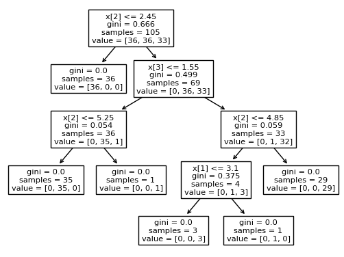
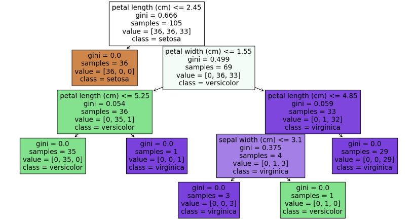
from sklearn.tree import export_graphviz
import matplotlib.pyplot as plt

export_graphviz(df_clf, out_file ='tree.dot',class_names = iris.target_names, feature_names = iris.feature_names, impurity =True, filled=True)
cl_list=list(iris.target_names)

import graphviz
fig = plt.figure(figsize=(15,8))
_=tree.plot_tree(df_clf,
              feature_names = iris.feature_names,
              class_names=cl_list,
              filled=True)
# 왼쪽이 참 오른쪽이 거짓 분할 기준
#정확도 측정
from sklearn.metrics import accuracy_score

pred = df_clf.predict(X_test)
ac1 = accuracy_score(y_test, pred)

print(ac1)
print(df_clf.get_params())

'''
0.9111111111111111
{'ccp_alpha': 0.0, 'class_weight': None, 'criterion': 'gini', 'max_depth': None, 'max_features': None, 'max_leaf_nodes': None, 'min_impurity_decrease': 0.0, 'min_samples_leaf': 1, 'min_samples_split': 2, 'min_weight_fraction_leaf': 0.0, 'random_state': 111, 'splitter': 'best'}
'''
의사결정트리 관련 실습 코드
2024_B.D.A_Data-Analysis-Modeling/Data_Analysis_Modeling/15주차 의사결정트리.ipynb at main · SeonHoYoo/2024_B.D.A_Data-
Contribute to SeonHoYoo/2024_B.D.A_Data-Analysis-Modeling development by creating an account on GitHub.
github.com